1. Why do we even do curve fitting on our data?
Curve fitting is the process of constructing a curve, or mathematical function, that has the best fit to a series of data points, possibly subject to constraints. [Wikipedia baaabaaaaay!]
Let’s say you conducted a simple tensile experiment (something similar to our Lab 1) on Captain America’s Vibranium shield (or, assume a very high strength Titanium rod if you haven’t watched Avengers).
As the Vibranium shield is very strong (way stronger than our testing machine), you report the stress strain measurements as below:
| Strain (microns) | Stress (kpa) |
|---|---|
| 0 | 0 |
| 1 | 10000 |
| 2 | 20000 |
| 3 | 30000 |
| 4 | 40000 |
| 5 | 50000 |
| 6 | 60000 |
| 7 | 70000 |
| 8 | 80000 |
| 9 | 90000 |
| 10 | 100000 |
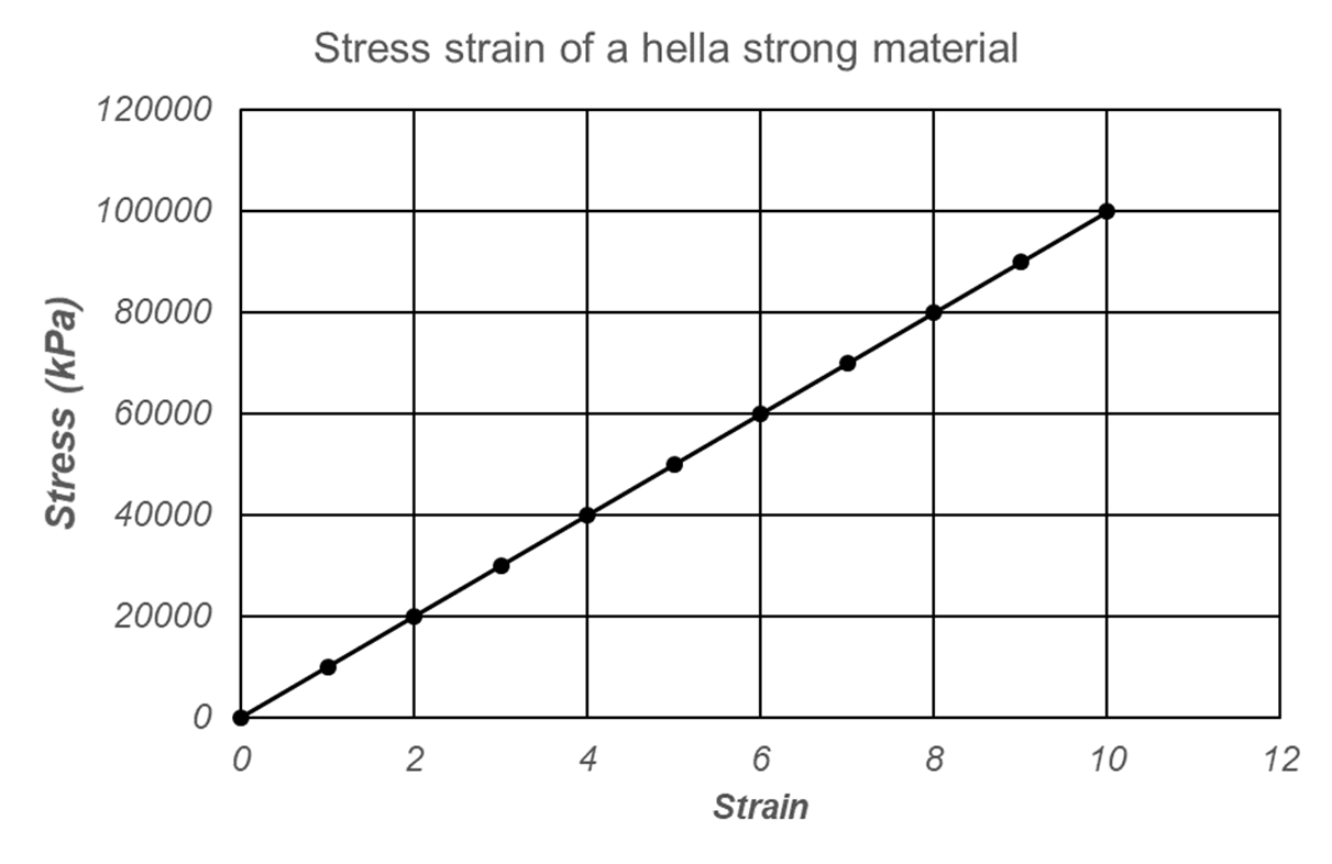
Looks great right? As the material is very strong and behaves elastically in all the strain ranges, the stress strain plot is a linear line.
Now think about this,
What if Thanos strikes the shield and produces a strain of 10000000 microns on our shield? Or, What if an earthquake hits a building made of this strong titanium material and induce a strain of 10000000000 microns?
The most obvious answer is, Let’s test our material to a strain of 10000000 or 10000000000.
Is that possible? Is there anything holding you back?
YES! THE TESTING MACHINE!!
Your testing machine is able to induce the maximum strain of 10. Any higher strain would break your testing machine (We don’t want that as UCD will ask you to pay for it, #sedlyf)
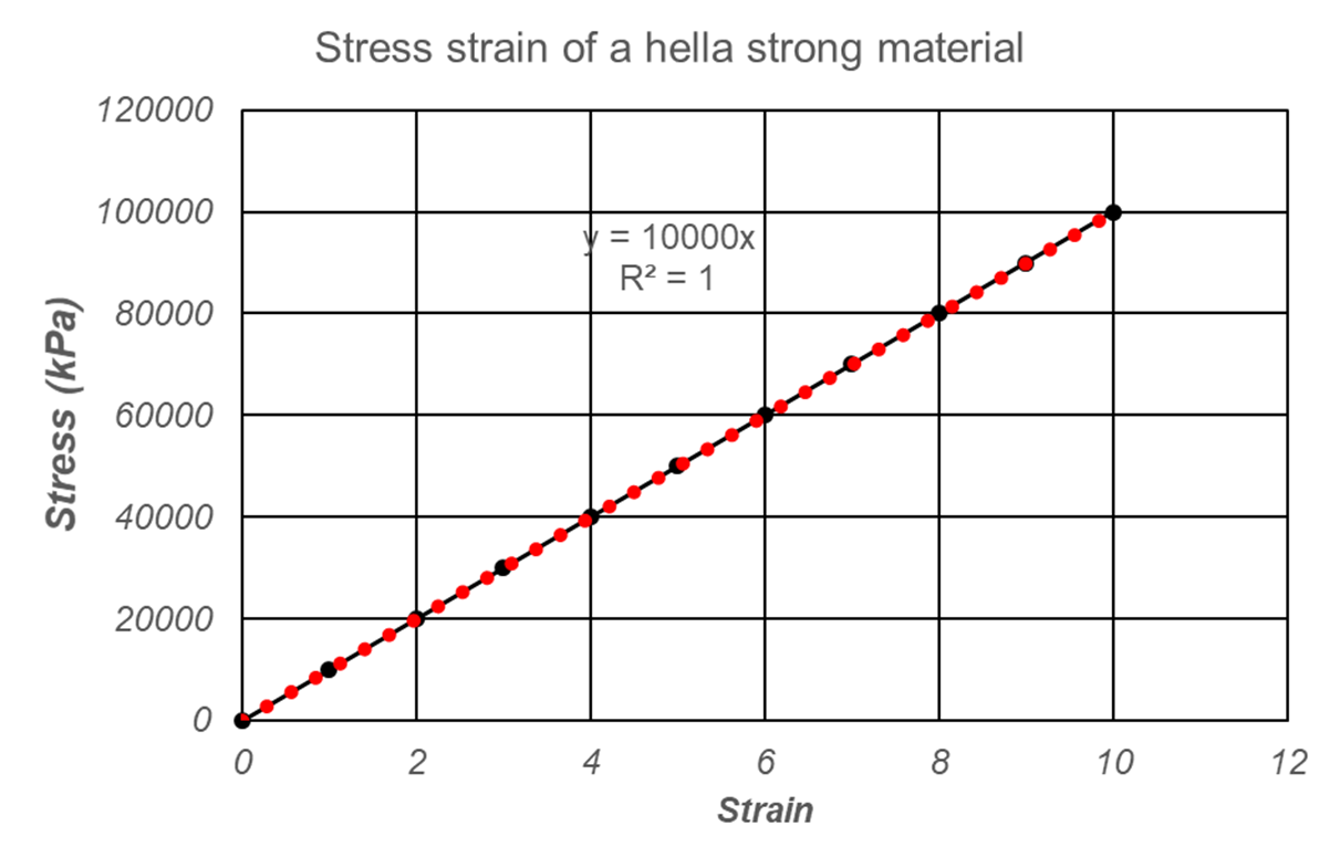
The next possible thing, that engineers love to do, is approximate the response using a curve or a line. The above graph looks like a straight linear line, so we can fit a straight line (y=mx+c) to our data. Fitting a line enables us “extrapolate” the data and approximate the stresses at very high strain levels.
You can use the basic excel trendline option to get a linear fit (shown in red dots in the figure below). Along with the red dot line, you get an equation of stress strain curve, which is:
$$ Stress = 10000\ x\ Strain $$
This equation is very powerful, as we can predict the stress at any strain. You can even use this equation to extrapolate the stress at very high strain, say 10000000000000. Just multiply your strain with 10000 and get the corresponding stress.
The design of all high rise buildings, and most engineering structures is done by Finite Element method (read about it for your discussion question). Finite element calculations are done on computers and computers LOOVVVEEE to work on equations. Researchers have produced complex “constitutive equations” (google it up or talk to me about it after the lab) for different materials which are directly used in the design and analysis of various structures using Finite Elements. These complex constitutive laws can predict the behavior of the material over a range of strain values and incorporate complex material behavior such as strain hardening, strain softening, fabric effects etc.
2. Why are we fitting a complex function to our lab 1 data?
For our test material in lab 1 (Mild Steel), the stress strain plot has an initial linear plot in the elastic region and a non-linear power law plot after the initial yield point. Due to that nonlinear bend we need a complex function to approximate the stresses for plastic deformation.
The initial elastic part can be approximated by a linear line (as shown in the first section of this document), but for this lab we are more interested in trying to find a curve that fits the non-linear or curved part after the initial yield point.
Luckily you are provided with a function that nicely fits the plastic region for our data. This equation is called the Ludwig’s equation and you can read more about it here.
$$ \sigma = \sigma_{y} + K \epsilon{p}^n $$
This equation is a non linear equation starting with a stress offset. How do we know it is non-linear? Whenever you have a something raised to the power and that power is not 1, the equation is essentially a non-linear equation. The n in the power generally varies between 0.2-0.5.
$$ \epsilon_p = \epsilon - \epsilon_0 $$
This equation gives the plastic deformation that occurs the body after the initial yield point.
So, what do these equation give you?
These equations essentially provide the stress corresponding to an input of the plastic strain experienced by the body. We can use them to extrapolate and model the internal stress with just knowing the plastic deformation caused by some loading. The parameters K and n control the shape of the non linear plot and the magnitude of the stress (play around and see what happens).
Remember as $ \epsilon_{p} $ will be negative below the initial yield point, you don’t need to worry about fitting the curve at strain below the initial yield point.
3. Steps to fit the lab 1 data
Find the yield stress and initial yield point. I have provided you the details how to get yield stress $\sigma_y$ and initial yield strain $\epsilon_0$.
Get the corresponding plastic strain for all the strain values beyond the initial yield strain.
Start with an initial value of K = Young’s Modulus/1500 and n=0.2
Use the equation to compute the corresponding stress value.
Plot the computed stress value with the original strain on the plot of experimentally measured stress and strain.
Play with K and n value to get a good fit.
4. Using the provided excel sheet
I am attaching an excel sheet which can help you get a feel for the fitting.
Excel Sheet to practice fitting
The data is some bogus/random data I created to help you out, so create a new sheet with the data from the experiment.
The different columns:
Strain data from the experiment
Stress data from the experiment
Plastic strain, you should remove all the -ve values
Stress from the equation, you should remove all the -ve values
Play with K and n to get a tight fitting between the computed and the measured results. Provide me with your fitted graph on the original graph along with the K and n values.