Introduction:
In the previous post, I tried to use inbuilt methods and a few libraries (Numpy and Pandas) to import our sensor data for subsequent processing.
In this post, I am going to use another spicy library for Python to plot our sensor data. Matplotlib is a plotting library with a spectrum of different user controls, which can be used to either quick plot your data or create publication quality plots. Matplotlib comes preinstalled for the Anaconda distribution, but if you don’t have it installed you can use:
 #For Anaconda command prompt
 conda install matplotlib
 #For pip
 pip install matplotlib
 # or
 python -m pip install -U pip
 python -m pip install -U matplotlib
To check which version of matplotlib you have, just type the following code in either Anaconda Prompt or terminal.
 python
 import matplotlib
 matplotlib.__version__
If the terminal prints a version, you are all set to go. I am going to use the pyplot API, which makes matplotlib work like MATLAB. Although matplotlib has another object-oriented API, but in most cases pyplot is more than sufficient. Before you can use matplotlib, you need to import the library by adding the following lines to your code:
import matplotlib.pyplot as plt
I am using the pandas read_csv method to import data and I am going to plot different columns with their names time s1 s2 s3 s4 s5 s6 s7, where s1 to s7 are different sensor numbers:
1. Simplest plot
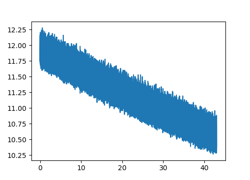
 plt.plot(df.time, df.s1)
 plt.show()
plt.plot is the simplest form of plot that produces a very basic line plot. The first argument is the x axis data (df.time) and the second argument is y axis data (df.s1). So, this line plots sensor1 data vs time data. To display the plot on the screen, plt.show() should always be added in the end.
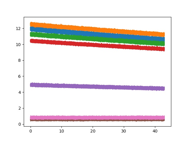
Let’s try plotting all the seven sensors data in a single plot.
 plt.plot(df.time, df.s1, df.time, df.s2, df.time, df.s3, df.time, df.s4,
             df.time, df.s4, df.time, df.s5, df.time, df.s6, df.time, df.s7)
 plt.show()
This is the most inefficient way of plotting all the sensor data on one plot, but Hey! it works. You have to define the x axis (df.time) again and again for every sensor number. The easier way would be to use a list and a for loop.
 list_of_sensors = ['s1','s2','s3','s4','s5','s6','s7']
 for sensor in list_of_sensors:
     plt.plot(df['time'], df[sensor])
 plt.show()
The list_of_sensors is a list containing the sensor numbers (in form of string) we want to plot. The for loop loops over this list and produces an iterator for each element in list. df[sensor] then uses the iterators and plots the sensor number on the plot. Once the for loop loops over all the sensor numbers the plot displays on the screen through plt.show().
2. Getting a little more control for your plots
Matplotlib was made with object-oriented approach at its heart, which provides superior control for your plots. First step is to use the subplots method to create a figure and axes object. The figure is the window in which plot is displayed and axes contains many arguments for our x-axis and y-axis manipulation. To create a simple figure object with axes use this code:
 fig,axes1 = plt.subplots(nrows=1,ncols=1)
 axes1.plot(df['time'] , df['s1'])
 plt.show()
The first line creates a figure object named fig which contains one axes names axes. The nrows and ncols argument can be used to define mutiple plots in a single figure (I will show you how to do that next). For now, as I am creating a single plot between time and sensor1, the number of rows and number of columns is just 1. By defining and naming an axes, you can directly call it to plot data on it using its name as axes1.plot instead of using plt.plot.
What if you want to plot data from all seven sensors in different subplots in same figure? Don’t worry, I gotchu!
 fig,axes = plt.subplots(nrows=3,ncols=3)
 # row = 1, column =1
 axes[0, 0].plot(df['time'], df['s1'])
 # row = 1, column =2
 axes[0, 1].plot(df['time'], df['s2'])
 # row = 1, column =3
 axes[0, 2].plot(df['time'], df['s3'])
 # row = 2, column =1
 axes[1, 0].plot(df['time'], df['s4'])
 # row = 2, column =2
 axes[1, 1].plot(df['time'], df['s5'])
 # row = 2, column =3
 axes[1, 2].plot(df['time'], df['s6'])
 # row = 3, column =2
 axes[2, 1].plot(df['time'], df['s7'])
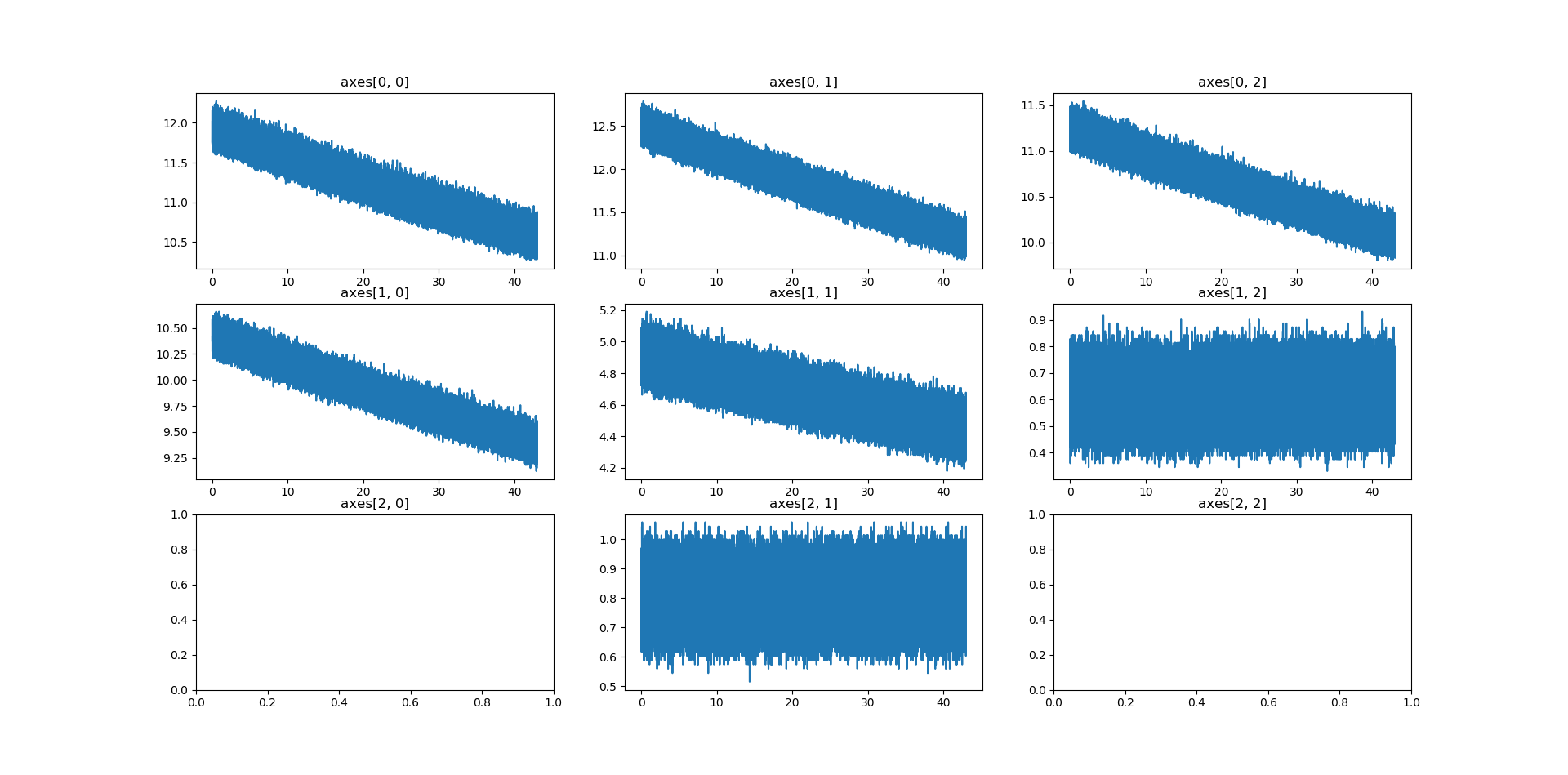
To plot data from all seven sensors, I defined a 9x9 axes matrix with 3 rows (nrows) and 3 columns (ncols). These axes can be accessed by their postion on the 9x9 matrix. As Python starts indexing at 0, the first axes for row 1 and column 1 is accessed as axes[0, 0]. Using the same indexing, the diagonal elements can be accessed as axes[0, 0] (row = 1, column = 1), axes[1, 1] (row = 2, column = 2), axes[2, 2] (row = 3, column = 3).
If you dont like the matrix way of accessing the subplots, there is another way to define this subplots grid. You can provide a name to each axes which makes accessing them easier. This is done by unpacking the subplots into a tuple and giving each element a name (axes1 to axes 9).
 fig,((axes1,axes2,axes3),
         (axes4,axes5,axes6),
         (axes7,axes8,axes9)) = plt.subplots(nrows=3,ncols=3)
 axes1.plot(df['time'],df['s1'])
 axes2.plot(df['time'],df['s2'])
 axes3.plot(df['time'],df['s3'])
 axes4.plot(df['time'],df['s4'])
 axes5.plot(df['time'],df['s5'])
 axes6.plot(df['time'],df['s6'])
 axes8.plot(df['time'],df['s7'])
As you can see in the figure above, I have total 9 subplots but I am plotting over just 7 of them. To deactivate and hide the unused subplots you can use axes.set_visible(False) argument. I don’t want the subplots at row number 3 and columns numbers 1 and 3 so I can either access them using the matrix notation or directly by the axes names.
 # Using matrix notation
 axes[2, 0].set_visible(False)
 axes[2, 2].set_visible(False)
 # Using axes names
 axes7.set_visible(False)
 axes9.set_visible(False)