Reusing your matplotlib setting

Different journals/conferences/universities could have different styles of figure/plots/graphs that you have to adhere to for your papers or reports. It makes sense to spend some time trying to play with matplolib, and try to recreate the same official template. Once you are happy with the outcome, you can store these settings in a .mplstyle file and import it whenever you need to plot something.

In this post, I am going to create a small .mplstyle style sheet file and try to recreate our publication quality plot from the previous post. The main idea is to use the matplotlib RcParams, from the matplotlib configuration API (add link), to configure our plot. These RcParams are called from a .mplstyle style sheet file and control the appearance of our plot. Although I am going to talk about the most commonly used parameters, you can find an extensive list of parameters at the official website.

1. Using the pre-defined style sheet

matplotlib already provides pre-defined style sheets to help you out with configuration. A complete list of pre-defined style sheets can be found here[]. To get a list of these available style, you can use:

import matplotlib.pyplot as plt
print(plt.style.available)      

['bmh', 'classic', 'dark_background', 'fast', 'fivethirtyeight', 'ggplot', 'grayscale', 'seaborn-bright', 'seaborn-colorblind', 'seaborn-dark-palette', 'seaborn-dark', 'seaborn-darkgrid', 'seaborn-deep', 'seaborn-muted', 'seaborn-notebook', 'seaborn-paper', 'seaborn-pastel', 'seaborn-poster', 'seaborn-talk', 'seaborn-ticks', 'seaborn-white', 'seaborn-whitegrid', 'seaborn', 'Solarize_Light2', 'tableau-colorblind10', '_classic_test']

Let’s try to plot the sensor data using the grayscale style sheet. To use any of these available styles, you need to add this line on top of your python script:

plt.style.use('grayscale')

The plot would change into grayscale and be something like this:

2. Defining the .mplstyle style sheet file

I am going to go through my ‘journalXYZ.mplstyle’ style sheet to walk you through the different segments I use to recreate the publication quality plot.

a. Font family

font.family     :   arial

This parameters defines the global font family for different texts in the plots, which could either be the axes labels, tick labels, legend, axes title, or any other text added to the plot. You can add other font parameters, like fontstyle, fontweight etc etc on a global figure level.

b. Line parameters

line.linewidth     :   1

This parameter changes the linewidth of the plotted data lines so that they dont look too thick!!!

c. Tick Paramters

Ticks are the tick marks on the axes (small lines above the numerical values) which show specific quantities.

# x tick paramters
xtick.direction     :   in
xtick.top           :   True
xtick.bottom        :   True
xtick.minor.visible :   True
xtick.labelsize     :   18

# y tick paramters
ytick.direction     :   in
ytick.left          :   True
ytick.right         :   True
ytick.minor.visible :   True
ytick.labelsize     :   18

Let’s go over these parameters one by one:

1. ().direction controls the tick direction which could either be inwards towards the center (in), outwards (out) or in both direction (both).
2. xticks.top, xticks.bottom, yticks.left, yticks.right controls the visibility of the ticks on the top, bottom,left and right axes of the figure.
   
3. ().minor.visible controls the visibility of the minor ticks.
4. ().labelsize controls the font size of the tick labels, which can be numbers (like ‘[0,10,20,30,40,50]‘) or strings.

d. Axes label parameters

Axes labels are the names given to the quantities on the x axis (Time) and y axis (Sensor data).

axes.labelweight    :   bold
axes.labelsize      :   22 
axes.labelpad       :   15.0 

Let’s go over these parameters one by one:

1. axes.labelweight controls the thickness of numerical value on the axis (or strings) and adds boldness tothe labels.
2. axes.labelsize controls the font size of the labels.
3. axes.labelpad controls the distance between the axes tick labels and axes labels, say between [0,10,20,30,4050] and ‘Time’ on the x axis.

e. Legend parameters

The final set of parameters to add are the legend parameters.

legend.loc          :   upper right
legend.fontsize     :   12
legend.edgecolor    :   black
legend.framealpha   :   1

Let’s go over these parameters one by one:

1. legend.loc defines the position of the legend and you can find a list of the locations in my previous post orthe official document ()
2. legend.fontsize controls the font size of the labels in the legend
3. legend.edgecolor defines the border color for the legend with a border
4. legend.framealpha controls the transparency of the legend with transparency decreasing from value of 0 to 1.

The final step is to save the config file using .mplstyle extension. You can store this file anywhere in your system or use matplotlib config location (AppData/.matplotlib). You can find different methods of saving your stylesheet in the official documentation.

(Funny enough, I saved my file as ‘journal.mplstyle.txt’ and calling it actually worked! I might get to the bottom of this in some future post)

3. Importing our custom ‘journal.mplstyle’ style sheet

Add this line on the top of your plotting script to import your style sheet:

import matplotlib.pyplot as plt
plt.style.use(r"J:\journal.mplstyle") # Insert your save location here

plt.style.use will import our custom style sheet and apply to all the plots prepared in the script

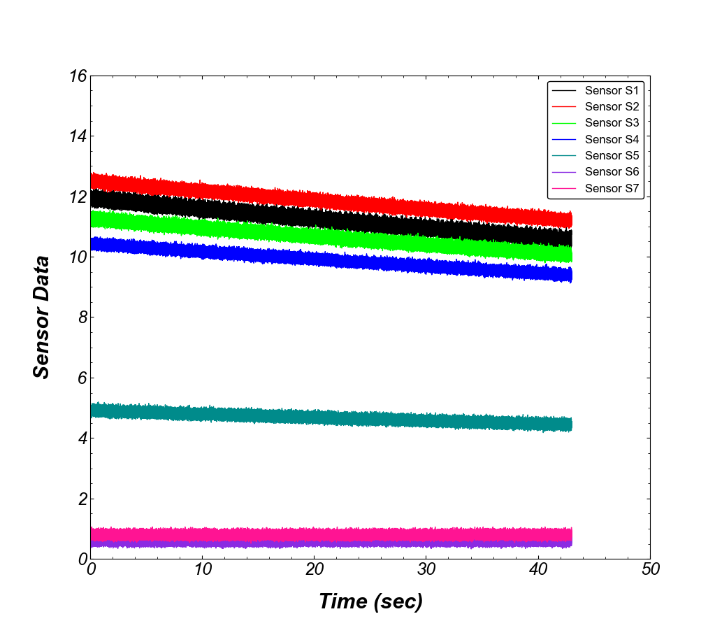
4. Plotting the sensor data

The final step is to actually plot something to see if our style sheet works,

    fig1,ax1 = plt.subplots(nrows=1,ncols=1,figsize=(10.33,9))
    list_of_sensors = ['s1','s2','s3','s4','s5','s6','s7']
    list_of_colors = ['black','r','lime','b','darkcyan','blueviolet','deeppink']
    list_of_labels = ['Sensor S1','Sensor S2','Sensor S3','Sensor S4','Sensor S5','Sensor S6','Sensor S7']
    
    for i,j in enumerate(list_of_sensors):
        ax1.plot(df['time'],df[j],
                color=list_of_colors[i],
                label=list_of_labels[i])
    
    ax1.set_xlim(0,50,10)
    ax1.set_ylim(0,16,2)
    ax1.set_xlabel('Time (sec)')
    ax1.set_ylabel('Sensor Data')
    ax1.legend()
    plt.show()

If you compare the above snippet with the code from last post, we saved a lot of trouble writing different parameters for labels, ticks, legends etc etc.

This method of saving and importing your matplotlib settings saves the time and effort required to plot, and can help in automating a lot of stuff.

Hope this post helped you in defining, saving and importing the perfect plot settings!