Introduction
The data from the experiments or simulations, exists as discrete numbers which I usually store as text or binary files. Let’s see the data from one of my experiments:
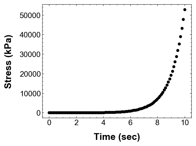
As soon as I see this data, I can tell that there is a non-linear (maybe exponential) relationship between time and stress. Wouldn’t it be awesome if I could fit a line through this data so that I can predict/extrapolate the stress value at any given time? Well, one of the prime tasks in geotechincal engineering is trying to fit meaningful relationships to sometimes quite absurd and random data.
The easiest way to fit a function to a data would be to import that data in Excel and use its predefined Trendline function. The Trendline option is quite robust for common set of function (linear, power, exponential etc) but it lacks in complexity and rigorosity often required in engineering applications. This is where our best friend Python comes into picture.
In this tutorial, we will look into:
1. scipy’s curve_fit module
2. lmfit module (which is what I use most of the time)
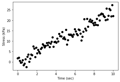
1. Generate data for a linear fitting
Let’s generate some data whose fitting would be a linear line with equation: \begin{equation} y = m x + c \end{equation}
where, m is usually the slope of the line and c is the intercept when x = 0 and x (Time), y (Stress) is our data. The y axis data is usually the measured value during the experiment/simulation and we are trying to find how the y axis quantity is dependent on the x axis quantity.
# Importing numpy for creating data and matplotlib for plotting
import numpy as np
import matplotlib.pyplot as plt

# Creating x axis data
x = np.linspace(0,10,100)

# Creating random data for y axis
# Here the slope (m) is predefined to be 2.39645
# The intercept is 0
# random.normal method just adds some noise to data
y = 2.39645 * x + np.random.normal(0, 2, 100)

# Plotting the data
plt.scatter(x,y,c='black')
plt.xlabel('Time (sec)')
plt.ylabel('Stress (kPa)')
plt.show()
2. Using Scipy’s curve_fit module
Scipy has a powerful module for curve fitting which uses non linear least squares method to fit a function to our data. The documentation is available it https://docs.scipy.org/doc/scipy/reference/generated/scipy.optimize.curve_fit.html.
To use curve_fit for the above data, we need to define a linear function which will be used to find fitting. The output will be the slope (m) and intercept ( c ) for our data, along with any variance in these values and any fitting statistics ($R^2$ or $\chi^2$).
# Calling the scipy's curve_fit function from optimize module
from scipy.optimize import curve_fit

# Defining a fitting fucntion
def linear_fit(x,m,c):
    return m*x + c

'''
1. Using the curve_fit function to fit the random linear data
2. Params returns an array with the best for values of the different fitting parameters. In our case first entry in params will be the slope m and second entry would be the intercept.
3. Covariance returns a matrix of covariance for our fitted parameters.
4. The first argument f is the defined fitting function.
5. xdata and ydata are the x and y data we generated above.
'''
params, covariance = curve_fit(f = linear_fit, xdata = x, ydata = y)

print('Slope (m) is ', params[0])
print('Intercept (c) is ', params[1])
print(covariance)
Slope (m) is  2.430364409972301
Intercept (c) is  -0.11571245549643683
[[ 0.00434152 -0.02170757]
 [-0.02170757  0.14544807]]
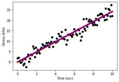
The slope of the line provided by curve_fit is lower/higher than the input slope. This is due to the random noise introduced in the data. Also, due to this noise the intercept is non zero.
What if we want the line to pass through origin (x=0,y=0)? In other words, what if we want the intercept to be zero?
We can force the curve_fit to works inside the bounds defined by you for the different fitting parameters. Let’s force the intercept ( c ) to be zero, and slope (m) to work between 1 and 3.
Also, let’s plot the two set of fitted parameters we obtained along with the data we generated.
'''
1. Bounds argument provides the bounds for our fitting parameters.
2. The format for bounds is ((lower bound of m, lower bound of c),(upper bound of m, upper bound of c))
3. curve_fir doesn't have an argument to make a parameter fixed, so I gave a very small value to c to force is close to 0.ArithmeticError
'''

params2, covariance2 = curve_fit(f = linear_fit, xdata = x, ydata = y, bounds=((2,0),(3,0.00000001)))

print('Slope (m) is ', params2[0])
print('Intercept (c) is ', params2[1])
print(covariance2)

plt.scatter(x,y,c='black')
plt.xlabel('Time (sec)')
plt.ylabel('Stress (kPa)')
plt.plot(x, linear_fit(x,params[0],params[1]),c='red',ls='-',lw=5)
plt.plot(x, linear_fit(x,params2[0],params2[1]),c='blue',ls='-',lw=2)
plt.show();
Slope (m) is  2.4130947618073093
Intercept (c) is  9.39448469276871e-15
[[ 0.0043456  -0.02172798]
 [-0.02172798  0.14558476]]
What if we want some statistics parameters ($R^2$)?
Although covariance matrix provides information about the variance of the fitted parameters, mostly everyone uses the standard deviation and coefficient of determination ($R^2$) value to get an estimate of ‘goodness’ of fit. I use it all the time for simpler fittings (linear, exponential, power etc).
# Getting the standard deviation
standarddevparams2 = np.sqrt(np.diag(covariance2))

# Getting the R^2 value for the fitting
# Read more at https://en.wikipedia.org/wiki/Coefficient_of_determination

# Step 1 : Get the residuals for fitting
residuals = y - linear_fit(x,params2[0],params2[1])

# Step 2 : Get the sum of squares of residual
squaresumofresiduals = np.sum(residuals**2)

# Step 3 : Get the total sum of squares using the mean of y values
squaresum = np.sum((y-np.mean(y))**2)

# Step 4 : Get the R^2
R2 = 1 - (squaresumofresiduals/squaresum)


print('The slope (m) is ', params2[0],'+-', standarddevparams2[0])
print('The intercept (c) is ', params2[1],'+-', standarddevparams2[1])
print('The R^2 value is ', R2)
The slope (m) is  2.4130947618073093 +- 0.06592113029190362
The intercept (c) is  9.39448469276871e-15 +- 0.3815557049874131
The R^2 value is  0.9327449525970685
Well the $R^2$ value for our is < 1, so it is not a good fit (although 0.9 is not bad, all depends on what you are looking for). Now look at the standard deviation on the intercept. Scipy’s curve_fit is not able to accurately force the intercept to be zero which causes that high standard deviation and a low $R^2$ value.
This is where lmfit (my favorite fitting package) comes into play. As the complexity of fitting function and parameter bounds increases curve_fit becomes less accurate and more crumbersome.
2. Using lmfit module
Lmfit provides a high-level interface to non-linear optimization and curve fitting problems for Python. It builds on and extends many of the optimization methods of scipy.optimize, has been quite mature and provides a number of useful enhancements and quality of life improvements.
The most welcomed feature is the parameter and results classes, which along with the minimize function provides a seamless pythonic way for any curve fitting needs. Personally, I love it and have been using it for couple of years for many many curve fittings in different coordinate systems. With lmfit I can clearly and concisely define my fitting functions and parameter bounds and display quite a lot of statistical data for my fit.
Let’s try our linear fitting using lmfit!
'''
1. Importing the module. If you dont have lmfit, you can download it on pip or conda. Instructions at https://lmfit.github.io/lmfit-py/installation.html
2. Parameters is the main parameters class.
3. minimize is the main fitting function. Takes our parameters and spits the best fit parameters.
4. fit_report provides the parameter fit values and different statistical values.
'''

from lmfit import Parameters,minimize, fit_report

# Define the fitting function
def linear_fitting_lmfit(params,x,y):
    m = params['m']
    c = params['c']
    y_fit = m*x + c
    return y_fit-y

# Defining the various parameters
params = Parameters()
# Slope is bounded between min value of 1.0 and max value of 3.0
params.add('m', min=1.0, max=3.0)
# Intercept is made fixed at 0.0 value
params.add('c', value=0.0, vary = False)

# Calling the minimize function. Args contains the x and y data.
fitted_params = minimize(linear_fitting_lmfit, params, args=(x,y,), method='least_squares')

# Getting the fitted values
m = fitted_params.params['m'].value
c = fitted_params.params['c'].value

# Printing the fitted values
print('The slope (m) is ', m)
print('The intercept (c) is ', c)

# Pretty printing all the statistical data
print(fit_report(fitted_params))
The slope (m) is  2.4130947619915073
The intercept (c) is  0.0
[[Fit Statistics]]
    # fitting method   = least_squares
    # function evals   = 7
    # data points      = 100
    # variables        = 1
    chi-square         = 362.059807
    reduced chi-square = 3.65716977
    Akaike info crit   = 130.663922
    Bayesian info crit = 133.269093
[[Variables]]
    m:  2.41309476 +/- 0.03303994 (1.37%) (init = 1)
    c:  0 (fixed)
Seems a lot of work for a simple linear fitting?
Trust me, as soon as your fitting functions become complex you will run towards lmfit with its concise and powerful way of defining and bounding parameters.
Sometimes you need to look beyond just least squares ;)
3. Power law curve fitting
Power law fitting is probably one of the most common type of fitting in engineering. Most engineering parameters saturate after some time which is captured by a decreasing power function. The basic equation is described as:
\begin{equation} y = a x^b \end{equation}
The best example would be the change in area of a square relative to the change in the length of the square. The area of a square is dependent on its length as:
\begin{equation} \text{Area} = \text{Length}^2 \end{equation}
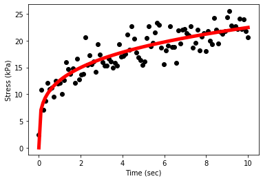
I frequently use power law to study the variation of stiffness with stress and create constitutive laws for materials. Let’s see how to do a power fitting with scipy’s curve_fit and lmfit.
# Creating a random dummy data for our power fittin
# a = 12.56
# b = 0.25
x = np.linspace(0,10,100)
y = 12.56 * x ** 0.25 + np.random.normal(0, 2, 100)

# Defining fitting function for curve_fit
def power_fit(x,a,b):
    return a * x ** b

# Calling the curve_fit function
params, covariance = curve_fit(f = power_fit, xdata = x, ydata = y)

print('a is ', params[0])
print('b is ', params[1])
print(covariance)

plt.scatter(x,y,c='black')
plt.xlabel('Time (sec)')
plt.ylabel('Stress (kPa)')
plt.plot(x, power_fit(x,params[0],params[1]),c='red',ls='-',lw=5)
plt.show();
a is  12.582417620337397
b is  0.25151997896349065
[[ 0.13306355 -0.00554453]
 [-0.00554453  0.00026803]]
from lmfit import Parameters,minimize, fit_report

# Define the fitting function
def power_fitting_lmfit(params,x,y):
    a = params['a']
    b = params['b']
    y_fit = a* x **b
    return y_fit-y

# Defining the various parameters
params = Parameters()
# Slope is bounded between min value of 1.0 and max value of 3.0
params.add('a', min= 1.0, max= 23.0)
# Intercept is made fixed at 0.0 value
params.add('b', min= 0.0, max= 1.0)

# Calling the minimize function. Args contains the x and y data.
fitted_params = minimize(power_fitting_lmfit, params, args=(x,y,), method='least_squares')

# Getting the fitted values
a = fitted_params.params['a'].value
b = fitted_params.params['b'].value

# Printing the fitted values
print('The a is ', a)
print('The b is ', b)

# Pretty printing all the statistical data
print(fit_report(fitted_params))

plt.scatter(x,y,c='black')
plt.xlabel('Time (sec)')
plt.ylabel('Stress (kPa)')
plt.plot(x, a*x**b,c='red',ls='-',lw=5)
plt.show();
The a is  12.582417884599595
The b is  0.25151996619258815
[[Fit Statistics]]
    # fitting method   = least_squares
    # function evals   = 11
    # data points      = 100
    # variables        = 2
    chi-square         = 380.338017
    reduced chi-square = 3.88100017
    Akaike info crit   = 137.589019
    Bayesian info crit = 142.799359
[[Variables]]
    a:  12.5824179 +/- 0.36477882 (2.90%) (init = 1)
    b:  0.25151997 +/- 0.01637166 (6.51%) (init = 0)
[[Correlations]] (unreported correlations are < 0.100)
    C(a, b) = -0.928

4. Transcendental function fitting
Let’s try a slightly complex function this time. Assume you have a sine wave, but it is decreasing in time. This happens when your oscillator loses it’s energy faster than it can provide, giving us a dampled sine wave. The equation of a damped sine wave is:
\begin{equation} y(t) = A e^{(-\lambda t)} cos(\omega t +\phi) \end{equation}
where, A is the amplitude of wave, $\lambda$ is the decay constant, $\omega$ is the angular frequency and $\phi$ is the phase angle. This is super simple with the lmfit module.
# Creating a random dummy data for our power fittin
# A = 2.5
# lambda = 0.5
# omega = 7.2
# phi = 3.14
t = np.linspace(0,6,100)
y = 2.5*np.exp(-0.5*t)*np.cos(7.2*t+3.14) + np.random.normal(0, 0.25, 100)

# Define the fitting function
def decaying_sine(params,t,y):
    A = params['A']
    lambdas = params['lambdas'] #lambda has a different meaning in python
    omega = params['omega']
    phi = params['phi']
    y_fit = A * np.exp(-lambdas*t)*np.cos(omega*t+phi)
    return y_fit-y

# Defining the various parameters
params = Parameters()
params.add('A', min= 1.0, max= 5.0)
params.add('lambdas', min= -1.0, max= 1.0)
params.add('omega', min= 0.0, max= 10.0)
params.add('phi', min= 0.0, max= 10.0)

# Calling the minimize function. Args contains the x and y data.
fitted_params = minimize(decaying_sine, params, args=(t,y,), method='nelder')

# Getting the fitted values
A = fitted_params.params['A'].value
lambdas = fitted_params.params['lambdas'].value
omega = fitted_params.params['omega'].value
phi = fitted_params.params['phi'].value

# Pretty printing all the statistical data
print(fit_report(fitted_params))

plt.scatter(t,y,c='black')
plt.xlabel('Time (sec)')
plt.ylabel('Stress (kPa)')
plt.plot(t, A * np.exp(-lambdas*t)*np.cos(omega*t+phi),c='red',ls='-',lw=5)
plt.show();
[[Fit Statistics]]
    # fitting method   = Nelder-Mead
    # function evals   = 357
    # data points      = 100
    # variables        = 4
    chi-square         = 6.70880707
    reduced chi-square = 0.06988341
    Akaike info crit   = -262.174903
    Bayesian info crit = -251.754223
##  Warning: uncertainties could not be estimated:
    this fitting method does not natively calculate uncertainties
    and numdifftools is not installed for lmfit to do this. Use
    `pip install numdifftools` for lmfit to estimate uncertainties
    with this fitting method.
[[Variables]]
    A:        2.51443557 (init = 1)
    lambdas:  0.49479403 (init = -1)
    omega:    7.21220270 (init = 0)
    phi:      3.11888095 (init = 0)

Both scipy and lmfit are powerful curve fitting tools and hopefully this tutorial helps you in appreciating their power!